LimROTS: Survival Analysis with Cox and Competing Risks Models
Source:vignettes/LimROTS_survival.Rmd
LimROTS_survival.RmdIntroduction
LimROTS extends its reproducibility-optimized testing framework to
survival analysis via the LimROTS_survival() function. It
fits a Cox proportional hazards model Therneau
(2024) — or, optionally, a competing risks model via the
Fine–Gray subdistribution approach Gray
(2024) — per feature across bootstrap resamples. The
reproducibility-optimization step then selects the parameters
and
that maximize the overlap of top-ranked features over those resamples,
yielding:
where is the Cox model coefficient (log hazard ratio) and is its standard error for feature .
P-values are derived from permutation-based null distributions using
the qvalue package Storey et al.
(2024). This vignette demonstrates both models using a Crohn’s
disease gut microbiome dataset.
Citation
If you use LimROTS in your research, please cite:
Anwar, A. M., Jeba, A., Lahti, L., & Coffey, E. (2025). LimROTS: A Hybrid Method Integrating Empirical Bayes and Reproducibility-Optimized Statistics for Robust Differential Expression Analysis. Bioinformatics, btaf570. https://doi.org/10.1093/bioinformatics/btaf570
Dataset Description
We use the crohn_survival dataset from the
miaTime package Lahti et al.
(2024). This is a simulated dataset based on a real Crohn’s
disease microbiome study (Gevers et al. 2014; Calle et
al. 2023). It contains 150 individuals
and 48 gut microbial taxa stored as a
TreeSummarizedExperiment object.
The relevant colData columns are:
| Column | Description |
|---|---|
diagnosis |
Group label ("CD" = Crohn’s disease,
"Control") |
event |
Binary event indicator (1 = Crohn’s disease, 0 = censored) |
event_time |
Time to event or censoring (unitless) |
The analysis goal is to identify taxa whose abundance is associated with time to Crohn’s disease diagnosis.
Loading the Data
library(LimROTS, quietly = TRUE)
library(mia, quietly = TRUE)
library(miaTime, quietly = TRUE)
library(TreeSummarizedExperiment, quietly = TRUE)
library(BiocParallel, quietly = TRUE)
library(SummarizedExperiment, quietly = TRUE)
library(ggplot2, quietly = TRUE)
data("crohn_survival")
print(crohn_survival)
#> class: TreeSummarizedExperiment
#> dim: 48 150
#> metadata(0):
#> assays(1): counts
#> rownames(48): g__Turicibacter g__Parabacteroides ...
#>   f__Rikenellaceae_g__ g__Bilophila
#> rowData names(4): order family genus taxonomy_id
#> colnames(150): 1939.SKBTI.0678 1939.SKBTI.0516 ... 1939.SKBTI.0237
#>   1939.SKBTI.0253.a
#> colData names(4): sample_id event event_time diagnosis
#> reducedDimNames(0):
#> mainExpName: NULL
#> altExpNames(0):
#> rowLinks: NULL
#> rowTree: NULL
#> colLinks: NULL
#> colTree: NULL
crohn_survival is a
TreeSummarizedExperiment. We first apply the centered
log-ratio (CLR) transformation using mia::transformAssay(),
which stores the result as a named assay ("clr") alongside
the original counts. We then coerce to a plain
SummarizedExperiment as required by
LimROTS_survival():
crohn_survival <- transformAssay(
    crohn_survival,
    assay.type = "counts",
    method     = "clr",
    pseudocount = TRUE,
    name       = "clr"
)
#> The assay contains already only strictly positive values. It is not recommended to add pseudocountin such case. To force adding pseudocount you canprovide a numeric value for the pseudocount argument.
assayNames(crohn_survival)
#> [1] "counts" "clr"
taxa_names <- rownames(crohn_survival)
crohn_survival <- as(crohn_survival, "SummarizedExperiment")
# as() coercion can drop rownames; restore them
if (is.null(rownames(crohn_survival))) {
    rownames(crohn_survival) <- taxa_names
}
print(crohn_survival)
#> class: SummarizedExperiment
#> dim: 48 150
#> metadata(0):
#> assays(2): counts clr
#> rownames(48): g__Turicibacter g__Parabacteroides ...
#>   f__Rikenellaceae_g__ g__Bilophila
#> rowData names(0):
#> colnames(150): 1939.SKBTI.0678 1939.SKBTI.0516 ... 1939.SKBTI.0237
#>   1939.SKBTI.0253.a
#> colData names(4): sample_id event event_time diagnosis
Sample names in crohn_survival contain .
characters, which can cause issues in formula parsing. We replace them
with _ in both the assay column names and the
colData row names:
clean_names <- gsub("\\.", "_", colnames(crohn_survival))
colnames(crohn_survival) <- clean_names
rownames(colData(crohn_survival)) <- clean_names
# Rename event_time -> time as required by LimROTS_survival()
colnames(colData(crohn_survival))[
    colnames(colData(crohn_survival)) == "event_time"] <- "time"
Inspect the survival outcome distribution:
Cox Proportional Hazards Analysis
The standard Cox model tests each taxon for an association with time-to-event independently of any other covariates.
Running LimROTS_survival
set.seed(1234, kind = "default", sample.kind = "default")
crohn_cox <- LimROTS_survival(
    x           = crohn_survival,
    assay.type  = "clr",
    niter       = 30,    # use >= 1000 for real analyses
    K           = 10,     # number of top taxa
    meta.info   = c("time", "event"),
    formula.str = "~ Surv(time, event)",
    competing_risks   = FALSE,
    verbose           = FALSE
)
#> Data is SummarizedExperiment object
#> Assay: clr will be used
#> Sanity check completed successfully!
#> Using MulticoreParam (Unix-like OS) with two workers.
#> qvalue() failed (return NULL): missing values and NaN's not allowed if 'na.rm' is FALSE
Note:
niter = 30is used here to reduce build time. For production analyses, useniter = 1000or higher and increase the number of parallel workers via theBPPARAMargument:# Windows BPPARAM <- SnowParam(workers = 4) # Linux / macOS BPPARAM <- MulticoreParam(workers = 4) # Pass to LimROTS_survival(..., BPPARAM = BPPARAM)
Results
The results are appended to the rowData and
metadata slots of the returned
SummarizedExperiment.
cox_res <- data.frame(
    rowData(crohn_cox),
    row.names = rownames(crohn_cox)
)
head(cox_res[order(cox_res$pvalue), ])
#>                      statistics       pvalue qvalue FDR  exp_coef   BH.pvalue
#> g__Actinomyces        0.4097402 0.0003472222     NA   0 1.4211011 0.003333333
#> f__Gemellaceae_g__    0.3184780 0.0003472222     NA   0 1.3033357 0.003333333
#> g__Lachnospira        0.3245194 0.0003472222     NA   0 0.7613151 0.003333333
#> g__Granulicatella     0.3266076 0.0003472222     NA   0 1.3154138 0.003333333
#> g__Streptococcus      0.3690089 0.0003472222     NA   0 1.3544171 0.003333333
#> o__Clostridiales_g__  0.2836266 0.0010416667     NA   0 0.7889692 0.008333333
Volcano plot of log hazard ratios versus (q-value):
cox_res$significant <- cox_res$FDR < 0.05

ggplot(cox_res, aes(
    x     = log(exp_coef),
    y     = -log10(pvalue),
    color = significant
)) +
    geom_point(alpha = 0.7, size = 2) +
    geom_hline(
        yintercept = -log10(0.05),
        linetype   = "dashed",
        color      = "steelblue"
    ) +
    scale_color_manual(
        values = c("FALSE" = "grey60", "TRUE" = "firebrick"),
        labels = c("FALSE" = "FDR \u2265 0.05", "TRUE" = "FDR < 0.05")
    ) +
    labs(
        title = "LimROTS Survival \u2014 Cox Model",
        x     = "Log Hazard Ratio",
        y     = expression(-log[10](pvalue)),
        color = NULL
    ) +
    theme_bw(base_size = 12) +
    theme(legend.position = "top")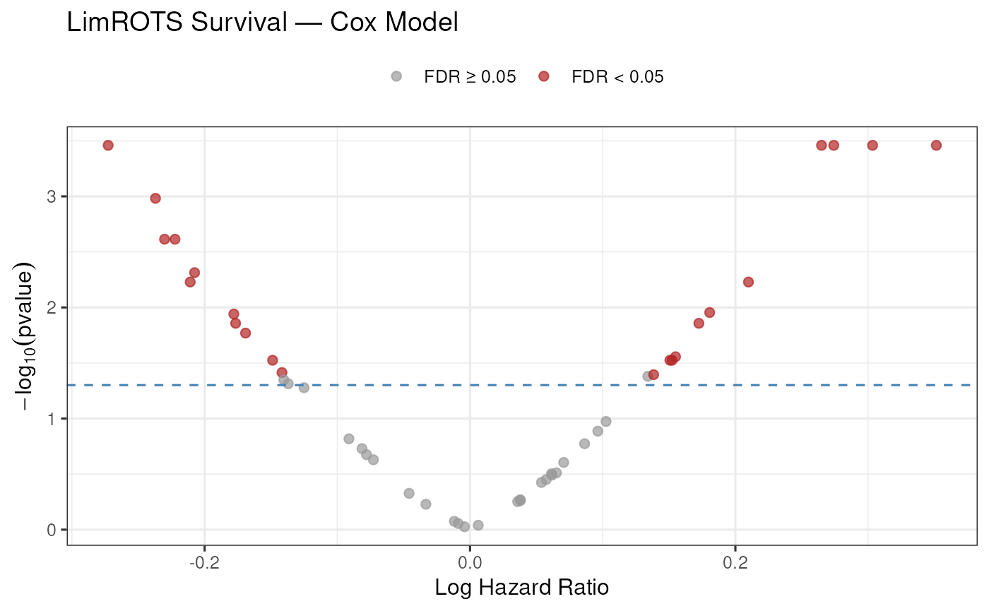
Competing Risks Analysis
When a competing event (e.g., death from another cause, remission)
prevents the event of interest from occurring, a competing risks model
is more appropriate than the standard Cox model.
LimROTS_survival() supports the Fine–Gray subdistribution
hazard model Gray (2024) when
competing_risks = TRUE.
The event variable must be coded as:
- 0 — censored
- 1 — event of interest
- 2 — competing event
Preparing the Data
The crohn_survival dataset has a binary event column
(0/1). For illustration, we recode half of the censored observations as
having experienced a competing event:
crohn_cr <- crohn_survival

event_vec <- colData(crohn_cr)$event
censored_idx <- which(event_vec == 0)

set.seed(42)
competing_idx <- sample(censored_idx, floor(length(censored_idx) / 2))
event_vec[competing_idx] <- 2L

colData(crohn_cr)$event <- event_vec
table(colData(crohn_cr)$event)
#>
#>  0  1  2
#> 38 75 37
Note: In a real study, the competing event column should reflect a genuine competing risk recorded in the original data (e.g., surgical intervention, withdrawal). The recoding above is purely for demonstration purposes.
Running LimROTS_survival
set.seed(1234, kind = "default", sample.kind = "default")
crohn_cr <- LimROTS_survival(
    x           = crohn_cr,
    assay.type  = "clr",
    niter       = 30,
    K           = 10,
    meta.info   = c("time", "event"),
    formula.str = "~ Surv(time, event)",
    competing_risks   = TRUE,
    verbose           = FALSE
)
#> Data is SummarizedExperiment object
#> Assay: clr will be used
#> Sanity check completed successfully!
#> Using MulticoreParam (Unix-like OS) with two workers.
Results
cr_res <- data.frame(
    rowData(crohn_cr),
    row.names = rownames(crohn_cr)
)
head(cr_res[order(cr_res$pvalue), ])
#>                     statistics       pvalue       qvalue FDR  exp_coef
#> g__Bacteroides        4.019771 0.0003472222 0.0006430041   0 0.8111478
#> g__Faecalibacterium   3.753486 0.0003472222 0.0006430041   0 0.8339016
#> g__Dialister          3.815381 0.0003472222 0.0006430041   0 1.1853826
#> g__Actinomyces        3.580579 0.0003472222 0.0006430041   0 1.4457244
#> f__Gemellaceae_g__    4.347935 0.0003472222 0.0006430041   0 1.3092273
#> g__Roseburia          3.941297 0.0003472222 0.0006430041   0 0.7931892
#>                       BH.pvalue
#> g__Bacteroides      0.001851852
#> g__Faecalibacterium 0.001851852
#> g__Dialister        0.001851852
#> g__Actinomyces      0.001851852
#> f__Gemellaceae_g__  0.001851852
#> g__Roseburia        0.001851852
Volcano plot for the competing risks model:
cr_res$significant <- cr_res$FDR < 0.05

ggplot(cr_res, aes(
    x     = log(exp_coef),
    y     = -log10(pvalue),
    color = significant
)) +
    geom_point(alpha = 0.7, size = 2) +
    geom_hline(
        yintercept = -log10(0.05),
        linetype   = "dashed",
        color      = "steelblue"
    ) +
    scale_color_manual(
        values = c("FALSE" = "grey60", "TRUE" = "firebrick"),
        labels = c("FALSE" = "FDR \u2265 0.05", "TRUE" = "FDR < 0.05")
    ) +
    labs(
        title = "LimROTS Survival \u2014 Competing Risks Model",
        x     = "Log Subdistribution Hazard Ratio",
        y     = expression(-log[10](pvalue)),
        color = NULL
    ) +
    theme_bw(base_size = 12) +
    theme(legend.position = "top")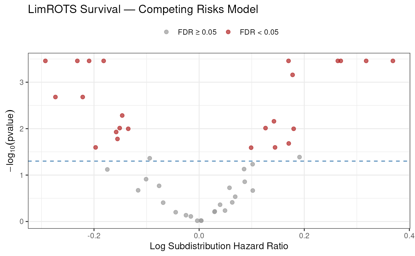
Quality Control
sessionInfo()
#> R version 4.6.0 (2026-04-24)
#> Platform: x86_64-pc-linux-gnu
#> Running under: Ubuntu 24.04.4 LTS
#>
#> Matrix products: default
#> BLAS:   /usr/lib/x86_64-linux-gnu/openblas-pthread/libblas.so.3
#> LAPACK: /usr/lib/x86_64-linux-gnu/openblas-pthread/libopenblasp-r0.3.26.so;  LAPACK version 3.12.0
#>
#> locale:
#>  [1] LC_CTYPE=en_US.UTF-8       LC_NUMERIC=C
#>  [3] LC_TIME=en_US.UTF-8        LC_COLLATE=en_US.UTF-8
#>  [5] LC_MONETARY=en_US.UTF-8    LC_MESSAGES=en_US.UTF-8
#>  [7] LC_PAPER=en_US.UTF-8       LC_NAME=C
#>  [9] LC_ADDRESS=C               LC_TELEPHONE=C
#> [11] LC_MEASUREMENT=en_US.UTF-8 LC_IDENTIFICATION=C
#>
#> time zone: UTC
#> tzcode source: system (glibc)
#>
#> attached base packages:
#> [1] stats4    stats     graphics  grDevices utils     datasets  methods
#> [8] base
#>
#> other attached packages:
#>  [1] ggplot2_4.0.3                   BiocParallel_1.45.0
#>  [3] miaTime_1.2.0                   mia_1.20.0
#>  [5] TreeSummarizedExperiment_2.20.0 Biostrings_2.80.0
#>  [7] XVector_0.52.0                  SingleCellExperiment_1.34.0
#>  [9] MultiAssayExperiment_1.38.0     LimROTS_1.4.0
#> [11] SummarizedExperiment_1.42.0     Biobase_2.72.0
#> [13] GenomicRanges_1.64.0            Seqinfo_1.2.0
#> [15] IRanges_2.46.0                  S4Vectors_0.50.0
#> [17] BiocGenerics_0.58.0             generics_0.1.4
#> [19] MatrixGenerics_1.24.0           matrixStats_1.5.0
#> [21] BiocStyle_2.40.0
#>
#> loaded via a namespace (and not attached):
#>   [1] RColorBrewer_1.1-3          jsonlite_2.0.0
#>   [3] magrittr_2.0.5              ggbeeswarm_0.7.3
#>   [5] farver_2.1.2                nloptr_2.2.1
#>   [7] rmarkdown_2.31              fs_2.1.0
#>   [9] ragg_1.5.2                  vctrs_0.7.3
#>  [11] DelayedMatrixStats_1.34.0   minqa_1.2.8
#>  [13] htmltools_0.5.9             S4Arrays_1.12.0
#>  [15] BiocNeighbors_2.6.0         broom_1.0.12
#>  [17] SparseArray_1.12.0          variancePartition_1.42.0
#>  [19] sass_0.4.10                 KernSmooth_2.23-26
#>  [21] bslib_0.10.0                htmlwidgets_1.6.4
#>  [23] desc_1.4.3                  DECIPHER_3.8.0
#>  [25] pbkrtest_0.5.5              plyr_1.8.9
#>  [27] cachem_1.1.0                igraph_2.3.0
#>  [29] lifecycle_1.0.5             cmprsk_2.2-12
#>  [31] iterators_1.0.14            pkgconfig_2.0.3
#>  [33] rsvd_1.0.5                  Matrix_1.7-5
#>  [35] R6_2.6.1                    fastmap_1.2.0
#>  [37] rbibutils_2.4.1             digest_0.6.39
#>  [39] numDeriv_2016.8-1.1         scater_1.40.0
#>  [41] irlba_2.3.7                 textshaping_1.0.5
#>  [43] vegan_2.7-3                 beachmat_2.28.0
#>  [45] labeling_0.4.3              mgcv_1.9-4
#>  [47] abind_1.4-8                 compiler_4.6.0
#>  [49] withr_3.0.2                 aod_1.3.3
#>  [51] S7_0.2.2                    backports_1.5.1
#>  [53] DBI_1.3.0                   viridis_0.6.5
#>  [55] gplots_3.3.0                MASS_7.3-65
#>  [57] rappdirs_0.3.4              DelayedArray_0.38.0
#>  [59] bluster_1.22.0              corpcor_1.6.10
#>  [61] permute_0.9-10              gtools_3.9.5
#>  [63] caTools_1.18.3              tools_4.6.0
#>  [65] vipor_0.4.7                 otel_0.2.0
#>  [67] beeswarm_0.4.0              ape_5.8-1
#>  [69] remaCor_0.0.20              glue_1.8.1
#>  [71] nlme_3.1-169                grid_4.6.0
#>  [73] cluster_2.1.8.2             reshape2_1.4.5
#>  [75] gtable_0.3.6                tidyr_1.3.2
#>  [77] BiocSingular_1.28.0         ScaledMatrix_1.20.0
#>  [79] ggrepel_0.9.8               pillar_1.11.1
#>  [81] stringr_1.6.0               yulab.utils_0.2.4
#>  [83] limma_3.68.0                splines_4.6.0
#>  [85] dplyr_1.2.1                 treeio_1.36.0
#>  [87] lattice_0.22-9              survival_3.8-6
#>  [89] DirichletMultinomial_1.54.0 tidyselect_1.2.1
#>  [91] scuttle_1.22.0              knitr_1.51
#>  [93] gridExtra_2.3               reformulas_0.4.4
#>  [95] bookdown_0.46               RhpcBLASctl_0.23-42
#>  [97] xfun_0.57                   statmod_1.5.1
#>  [99] stringi_1.8.7               lazyeval_0.2.3
#> [101] yaml_2.3.12                 boot_1.3-32
#> [103] evaluate_1.0.5              codetools_0.2-20
#> [105] tibble_3.3.1                qvalue_2.44.0
#> [107] BiocManager_1.30.27         cli_3.6.6
#> [109] systemfonts_1.3.2           Rdpack_2.6.6
#> [111] jquerylib_0.1.4             Rcpp_1.1.1-1.1
#> [113] EnvStats_3.1.0              parallel_4.6.0
#> [115] pkgdown_2.2.0               ecodive_2.2.6
#> [117] sparseMatrixStats_1.24.0    bitops_1.0-9
#> [119] lme4_2.0-1                  decontam_1.32.0
#> [121] viridisLite_0.4.3           mvtnorm_1.3-7
#> [123] tidytree_0.4.7              lmerTest_3.2-1
#> [125] scales_1.4.0                purrr_1.2.2
#> [127] crayon_1.5.3                fANCOVA_0.6-1
#> [129] rlang_1.2.0